Describe your data using Python
 This is the first of a series of articles that I will write to give a gentle introduction to statistics. In this article we will introduce some basic statistical concepts and learn how to use basic statistics to help you describe your data.
We will cover the following topics in this article:
- The difference between a population and a sample
- The difference between Descriptive and Inferential statistics
- Different types of variables
- Types of descriptive statistics
- Normal or Gaussian distribution
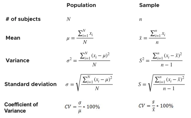
The difference between a population and a sample:
- Population denotes a large group consisting of elements having at least one common feature; it is the complete set of observations
- Sample is a finite subset of the population; it is a subset of observations from a population. We get a sample from the population in either of the following ways
- Representative sampling - here the sample’s characteristics are similar to the population characteristics - A simple random sample is the most common approach to obtain a representative sample - A systematic random sample - A cluster random sample - A stratified random sample
- Convenience sampling - here we collect sample from section of population that is easily available
The difference between Descriptive and Inferential statistics:
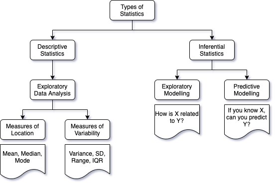
- Descriptive statistics - its all about organizing, describing and summarizing data
- Exploratory data analysis (EDA)
- measures of location - such as Mean, Median, Mode
- measures of variability or dispersion - such as Variance, Standard deviation, Range, Inter quartile range (IQR)
- Exploratory data analysis (EDA)
- Inferential statistics - its all about drawing conclusions about a population from analysis of a random sample drawn from the populaiton
- Exploratory modelling - how is x related to y?
- Predictive modelling - if you know x, can you predict y?
Different types of variables:
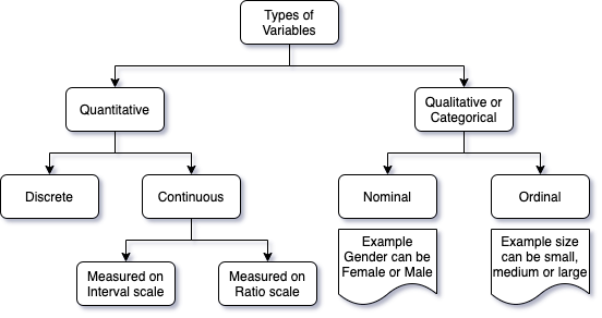
- Quantitative
- Discrete: a variable whose value is obtained by counting. Example, number of students in a class
- Continuous: a variable whose value is obtained by measuring. Example, height of all students in a class
- Interval: this is scale of measurement where continuous data is rank ordered
- Ratio: this is scale of measurement where continuous data is rank ordered + has meaningful spacing
- Qualitative or Categorical
- Nominal: example gender - female or male
- Ordinal: example size - small, medium, or large
Types of descriptive statistics:
- Measures of location: mainly measures of central tendency
- Mean: sum of all values divided by the number of values
import seaborn as sns tips = sns.load_dataset('tips') tips.mean() # shows mean of all numeric variables - Median: middle value in a given sequence of values ordered by rank
tips.median() # shows median of all numeric variables - Mode: most frequent value in a set of values
tips.mode() # shows mode of all variables
- Mean: sum of all values divided by the number of values
- Measures of variability, spread or dispersion
- Range: Maximum value - Minimum value
range = tips.total_bill.max() - tips.total_bill.min() # range - IQR (Inter quartile range): 75th percentile - 25th percentile
tips.total_bill.quantile(.75) - tips.total_bill.quantile(.25) # IQR - Variance: Measure of variability of data around the mean
tips.total_bill.var() # variance of total_bill variable - Standard deviation: how spread out the data is, i.e. how much variance there is from the mean
tips.total_bill.std() # standard deviation of total_bill variable - Coefficient of variance (C.V.): measure of standard deviation expressed as a percentage of the mean
cv = lambda x: x.std() / x.mean() * 100
cv(tips.total_bill)
- Range: Maximum value - Minimum value
- Measures of symmetry and peakedness: Skewness measures symmetry and Kurtosis measures peakedness
Normal or Gaussian distribution
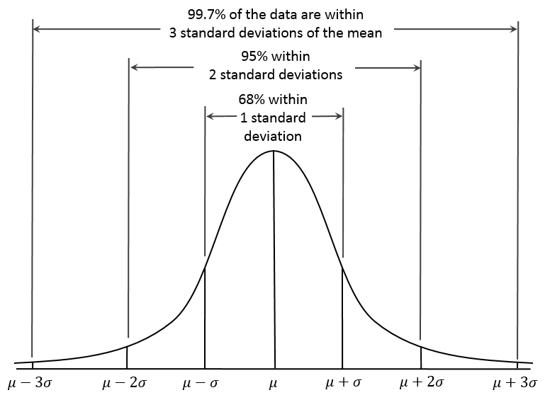
- This is one of the most common statistical distribution. The curve of this distribution is shaped like a bell.
- The shape of the bell depends on mean and standard deviation of the data
- Larger the standard deviation, wider the distribution
- A tip to quickly assess normality is to see if mean and median are nearly equal
Skewness and Kurtosis
- Skewness measures tendency of data to be spread out on one side of the mean than the other. Skewness value indicates
- Negative value indicates the data is left skewed
- Positive value indicates the data is right skewed
- Closer to zero for the data to be normally distributed
import scipy.stats as s
s.skew(tips.total_bill, bias=False)  #calculate sample skewness
- Kurtosis measures tendency of data to be concentrated around the center or tails. Kurtosis value indicates
- Platykurtic: Negative value indicates lower than normal peakedness
- Leptokurtic: Positive value indicates higher than normal peakedness
- Mesokurtic: Closer to zero for the data to be normally distributed
import scipy.stats as s
s.kurtosis(tips.total_bill, bias=False)  #calculate sample kurtosis
Comments welcome!